Finance environments
Six environments model the core problems of systematic trading. Each is a standard
sekai.Env (so wrappers, vector envs and the gymnasium bridge all apply), runs on simulated
prices by default, and comes with baselines, closed-form where the underlying model has one,
that a learned policy has to beat.
| ID | Problem | Model | Baseline |
|---|---|---|---|
Trading-v0 |
trade one asset | GBM, any market model, or your price history | buy and hold, momentum |
Portfolio-v0 |
allocate across assets and cash | correlated GBM, any market model, or your history | equal weight, inverse volatility |
Market-v0 |
trade a changing universe with costs, financing and outside data | two-regime market with listings and delistings, or your MarketData |
equal weight, a regime oracle |
MarketMaking-v0 |
quote a bid and an ask | Avellaneda & Stoikov (2008) | avellaneda_stoikov_action() |
OptimalExecution-v0 |
liquidate a large position | Almgren & Chriss (2000) | almgren_chriss_actions() |
LimitOrderBook-v0 |
quote and trade in a limit order book | zero-intelligence order flow | inventory-skewed quotes |
LimitOrderBookMarket puts several agents in one order book.
The first four have native vector versions that step
thousands of sub-envs at once. All of them are assembled from the
finance toolkit, whose parts (market models, cost models, reward
functions, metrics) they also accept as arguments.
Each has an RGB renderer in sekai.envs.finance that draws its episodes as a dashboard
(TradingRenderer, PortfolioRenderer, MarketRenderer, MarketMakingRenderer,
OptimalExecutionRenderer, LimitOrderBookRenderer and LimitOrderBookMarketRenderer):
the animations on this page, made by
examples/render_finance.py.
See Rendering for what each shows, and for building the same
kind of renderer for your own environment.
Rewards are additive over an episode: log growth of wealth for Trading-v0, Portfolio-v0
and Market-v0 (or any reward= you pass), risk-adjusted P&L for market making in both
its forms, and minus the implementation-shortfall objective (in basis points) for
execution. The horizon is part of each environment, so make() adds no TimeLimit.
Once an episode has ended (terminated or truncated), step() raises sekai.ResetRequired
until the next reset(), as it does before the first one; the vector versions reset
finished sub-envs themselves. Parameters are checked when the environment is built: a
negative volatility, a horizon, capital or price that is not positive, or a NaN raises
ValueError naming the parameter.
All baselines below are evaluated with one helper, over the same 200 seeds:
import numpy as np
import sekai
from sekai.envs.finance import simulate_gbm


def evaluate(env, policy, episodes=200):
    """Mean ± std of the episode return of policy(env, observation) over seeds 0..episodes-1."""
    totals = []
    for seed in range(episodes):
        result, total = env.reset(seed=seed), 0.0
        while not result.done:
            result = env.step(policy(env, result.observation))
            total += result.reward
        totals.append(total)
    return f"{np.mean(totals):+.4f} ± {np.std(totals):.4f}"
Your own price history
Trading-v0 and Portfolio-v0 accept historical closing prices through prices=:
a 1-D array (or a pandas Series) for Trading-v0, a (T, n_assets) array (or a pandas
DataFrame) for Portfolio-v0. A MarketData, with dates, asset
names and data fields, goes in data= instead, in these two environments as in
Market-v0 (below); a MarketData passed
as prices= raises TypeError. Give one source: prices=, data= or a model= to
simulate; more than one raises ValueError.
Every reset() then draws a random contiguous window of lookback + episode_length + 1
rows, so each episode starts at a different date. Prices must be finite and strictly
positive, and the history at least one window long; otherwise the constructor raises
ValueError.
prices = np.loadtxt("closes.csv", delimiter=",", skiprows=1, usecols=(1, 2, 3, 4))
env = sekai.make("Portfolio-v0", prices=prices, episode_length=126, lookback=20)
A pandas DataFrame or Series indexed by dates (a DatetimeIndex) keeps them: it is
converted with MarketData.from_pandas, so info["timestamp"] reports the dates, dt
follows their spacing and reset(options={"start": "2020-03-02"}) finds the date. With any
other index the rows are numbered from 0, as for an array.
import pandas as pd

closes = pd.read_csv("closes.csv", index_col=0, parse_dates=True)  # dates x tickers
env = sekai.make("Portfolio-v0", prices=closes, episode_length=126, lookback=20)
result = env.reset(seed=0, options={"start": "2020-03-02"})  # info["timestamp"]: 2020-03-02
The examples on this page use synthetic "histories" from simulate_gbm() (below) so that
they run offline; load real data the same way.
Trading-v0
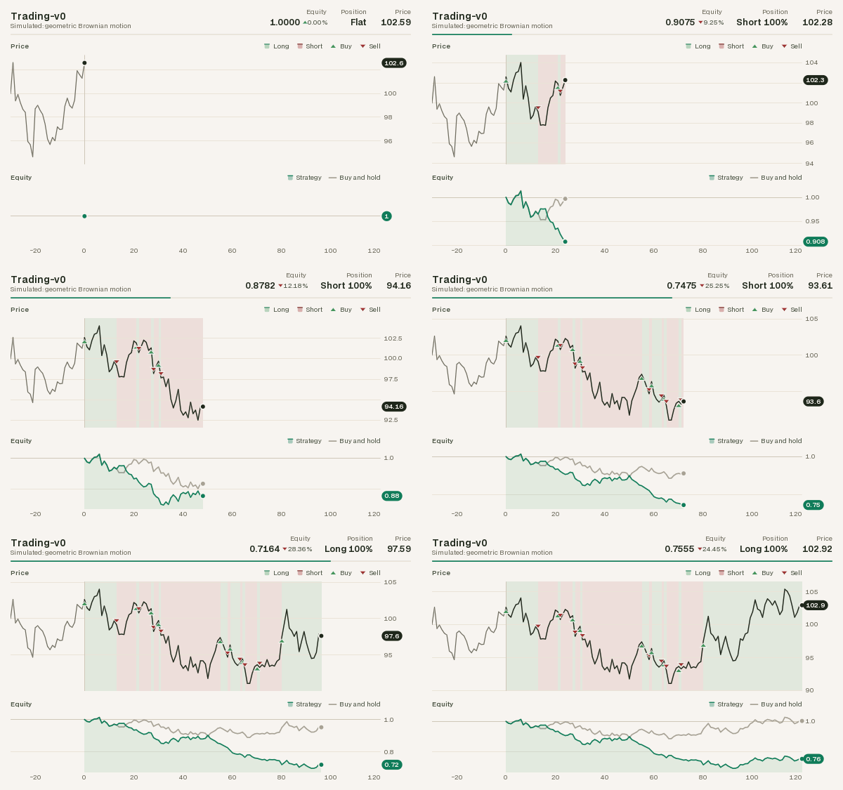
Trade a single asset by choosing a target position, as a fraction of equity, every step.
Dynamics. Without a history or a model, the price follows geometric Brownian motion,
simulated with the exact log-normal transition:
Choosing the target position \(w_t\) (from the positions grid) when the current position is
\(\tilde p_t\) costs \(c_t = \kappa\,\lvert w_t - \tilde p_t\rvert\) of equity, then the position
earns the asset's return \(r_{t+1} = S_{t+1}/S_t - 1\) and drifts with the price, exactly as a
one-asset Portfolio-v0 does:
The episode's total reward is therefore \(\log(W_T / W_0)\), the log return of the account. Holding a long (\(w = 1\)) or flat position costs nothing, since it does not drift; a short or levered position drifts away from its target as the price moves (a 100% short becomes \(-(1 + r)/(1 - r)\) of equity), and choosing the same target again trades the drift back and pays for it.
| Observation | Box(lookback + 1,) of float32: the last lookback log returns of the asset, then the current (drifted) position, bounded to [0, 1] when every target is in [0, 1] and unbounded below (above) when a target is short (above 1) |
| Action | Discrete(len(positions)): index into positions; the default (-1.0, 0.0, 1.0) is short / flat / long |
| Reward | \(\log g_t\), the log growth of equity net of costs |
| Termination | equity reaches zero (possible only with leverage or extreme moves) |
| Truncation | after episode_length steps (an episode is a window of an ongoing market, so time is not observed; add TimeAwareObservation if the policy should see it) |
info |
equity, position (\(\tilde p_{t+1}\)), price, asset_return, cost, turnover (\(\lvert w_t - \tilde p_t\rvert\)), timestamp, dt |
| Parameter | Default | Meaning |
|---|---|---|
prices |
None |
1-D historical prices (an array or a pandas Series); None simulates |
data |
None |
a one-asset MarketData instead of prices |
episode_length |
252 |
steps per episode (one trading year of days) |
lookback |
30 |
log returns in the observation |
positions |
(-1.0, 0.0, 1.0) |
allowed target positions, e.g. (0.0, 1.0) for long-only or (-2, -1, 0, 1, 2) for leverage |
transaction_cost |
1e-3 |
cost per unit of position change (\(\kappa\), here 10 bp), or any CostModel |
mu, sigma |
0.05, 0.2 |
GBM drift and volatility (annualised) |
dt |
None |
step length in years: 1 / data.periods_per_year on dated MarketData, else the model's dt, else 1/252 |
s0 |
100.0 |
initial simulated price |
model, reward, sampler, capital |
see options shared by Trading-v0 and Portfolio-v0 |
Baselines on ten years of daily history (a synthetic path with 6.3% annual drift and 20% volatility), one-year episodes, 20-day lookback:
history = simulate_gbm(np.random.default_rng(4), 2520, s0=100.0, mu=0.08, sigma=0.2)
log_returns = np.diff(np.log(history))
print(f"{log_returns.mean() * 252:.3f} {log_returns.std() * np.sqrt(252):.3f}")  # 0.063 0.199
env = sekai.make("Trading-v0", prices=history, episode_length=252, lookback=20)
SHORT, FLAT, LONG = 0, 1, 2
for name, policy in {
    "buy and hold": lambda env, obs: LONG,
    "flat": lambda env, obs: FLAT,
    "always short": lambda env, obs: SHORT,
    "momentum (20d)": lambda env, obs: LONG if obs[:-1].sum() > 0 else FLAT,
}.items():
    print(f"{name:15s} {evaluate(env, policy)}")
buy and hold    +0.0597 ± 0.2107
flat            +0.0000 ± 0.0000
always short    -0.1062 ± 0.2100
momentum (20d)  -0.0070 ± 0.1689
On a random walk there is nothing for momentum to find, so it gives up part of the drift and pays costs; a learned policy should at least match buy and hold on risk-adjusted terms. Always short also pays to keep its short at 100% of equity as the price drifts, about 0.5% a year here.
Portfolio-v0
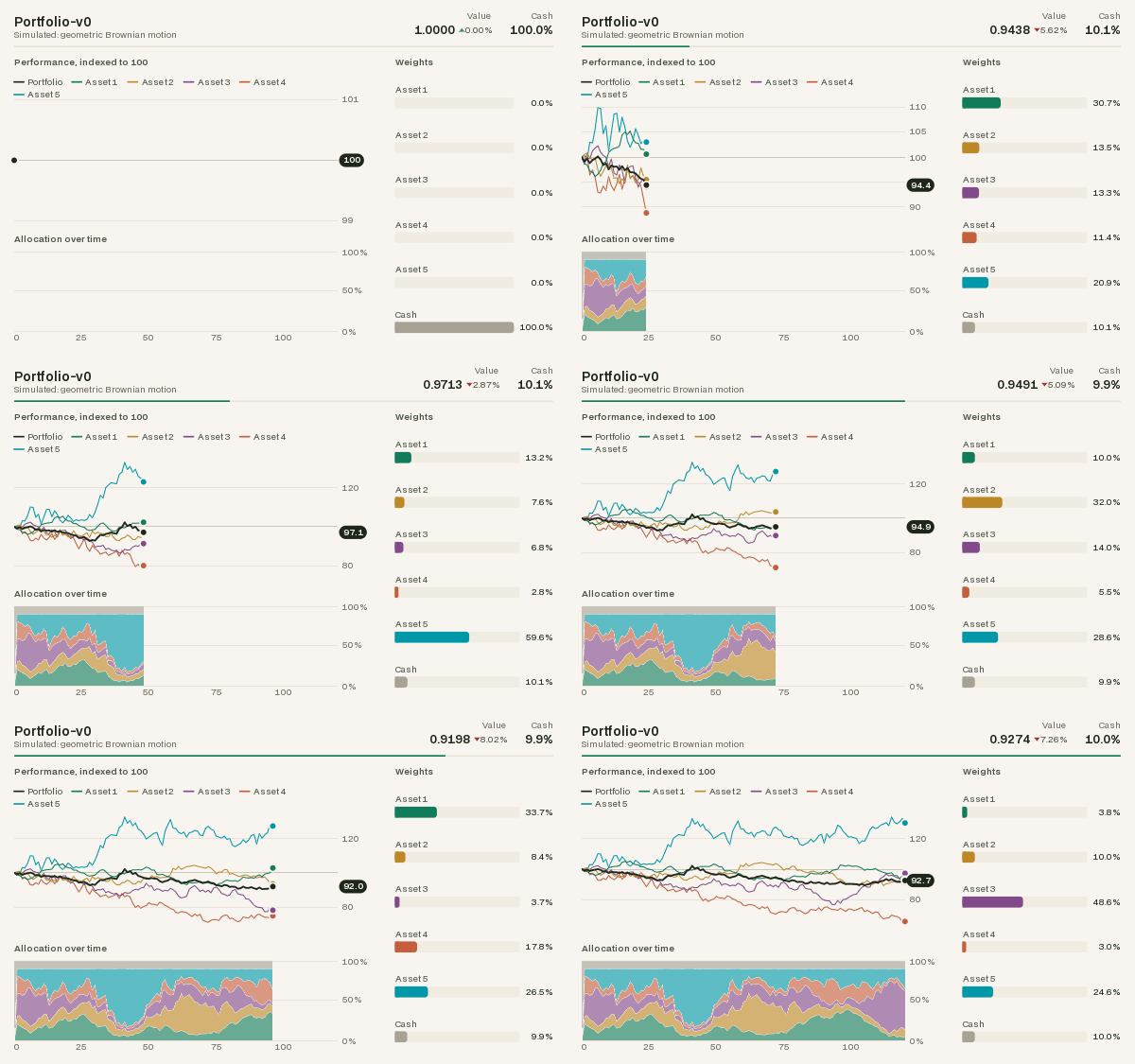
Allocate wealth across n_assets risky assets and cash, rebalancing every step.
Dynamics. Without a history or a model, asset prices follow correlated GBMs (as
above, with correlated shocks \(Z_t \sim \mathcal N(0, \Sigma)\)). The default market is fixed
across resets: drifts of 6%, volatilities spread evenly from 15% to 35%, and a fixed random
correlation matrix; only the path is random.
The action is mapped to target weights \(w_t\) over (assets, cash). Rebalancing from the drifted weights \(\tilde w_t\) has turnover \(\tau_t = \sum_{i=1}^{n} \lvert w_{t,i} - \tilde w_{t,i}\rvert\) (cash excluded) and costs \(c_t = \kappa\,\tau_t\):
with the cash return taken as zero. Summed over the episode the reward is the log growth of the portfolio.
| Observation | Dict: "returns", Box (lookback, n_assets) of recent log returns; "weights", Box (n_assets + 1,) of current (drifted) weights, cash last |
| Action (long-only, default) | Box(0, 1, (n_assets + 1,)) of scores, normalised to weights summing to 1, cash last; all zeros means all cash |
Action (allow_short=True) |
Box(-1, 1, (n_assets,)) of target asset weights, scaled down if gross exposure \(\sum_i \lvert w_i\rvert\) exceeds 1; the rest is cash |
| Reward | \(\log g_t\), log growth net of costs |
| Termination | portfolio value reaches zero (only possible with shorts) |
| Truncation | after episode_length steps (time is not observed, as in Trading-v0) |
info |
portfolio_value (also as equity), weights, turnover, cost, asset_returns, timestamp, dt |
env.unwrapped.action_to_weights(action) shows the mapping:
long_only = sekai.make("Portfolio-v0", n_assets=3)
print(long_only.action_to_weights(np.array([1, 1, 2, 0], np.float32)))  # [0.25 0.25 0.5  0.  ]

long_short = sekai.make("Portfolio-v0", n_assets=3, allow_short=True)
print(long_short.action_to_weights(np.array([0.8, -0.6, 0.2], np.float32)).round(3))  # [ 0.5   -0.375  0.125  0.75 ]
| Parameter | Default | Meaning |
|---|---|---|
prices |
None |
(T, n_assets) history (an array or a pandas DataFrame); None simulates |
data |
None |
a complete MarketData instead of prices |
n_assets |
None |
number of risky assets: 5 in the default simulation, else that of the history or model (a different value raises ValueError) |
episode_length |
252 |
steps per episode |
lookback |
30 |
rows of returns in the observation |
transaction_cost |
1e-3 |
cost per unit of turnover (\(\kappa\)), or any CostModel |
allow_short |
False |
switch to the long/short action space |
mu |
0.06 per asset |
annualised drifts (simulation) |
sigma |
linspace(0.15, 0.35, n_assets) |
annualised volatilities (simulation) |
corr |
fixed random | correlation matrix of the shocks (simulation) |
dt |
None |
step length in years: 1 / data.periods_per_year on dated MarketData, else the model's dt, else 1/252 |
model, reward, sampler, capital |
see options shared by Trading-v0 and Portfolio-v0 |
Baselines on ten years of history for four assets, one-year episodes, 60-day lookback:
corr = np.array([[1.0, 0.6, 0.3, 0.0],
                 [0.6, 1.0, 0.4, 0.1],
                 [0.3, 0.4, 1.0, 0.2],
                 [0.0, 0.1, 0.2, 1.0]])
prices = simulate_gbm(np.random.default_rng(0), 2520, s0=[50, 120, 30, 80],
                      mu=[0.08, 0.06, 0.12, 0.03], sigma=[0.25, 0.18, 0.4, 0.08], corr=corr)
env = sekai.make("Portfolio-v0", prices=prices, episode_length=252, lookback=60)


def inverse_volatility(env, obs):
    vol = obs["returns"].std(axis=0) + 1e-8
    return np.append(1 / vol, 0.0).astype(np.float32)


def buy_and_hold(env, obs):
    w = obs["weights"]  # after the first step, keeping the drifted weights costs nothing
    return np.ones(5, np.float32) if w[-1] == 1.0 else w


for name, policy in {
    "equal weight": lambda env, obs: np.ones(5, np.float32),
    "buy and hold": buy_and_hold,
    "inverse volatility": inverse_volatility,
    "all cash": lambda env, obs: np.eye(5, dtype=np.float32)[4],
}.items():
    print(f"{name:19s} {evaluate(env, policy)}")
equal weight        +0.1133 ± 0.1267
buy and hold        +0.1230 ± 0.1468
inverse volatility  +0.0913 ± 0.0954
all cash            +0.0000 ± 0.0000
Equal weight here rebalances daily (paying costs on the drift); inverse volatility gives up
some return for a markedly lower dispersion. For an MLP policy, flatten the observation with
FlattenObservation (and consider TimeAwareObservation); SB3 users can keep the Dict
with MultiInputPolicy (example).
Options shared by Trading-v0 and Portfolio-v0
Both environments take these arguments too. Left at their defaults, the environments
behave exactly as described above. episode_length and lookback (here and in
Market-v0) size the env's arrays, so they are read-only after construction: setting them,
directly or through a vector env's set_attr, raises AttributeError; make a new env instead.
| Parameter | Default | Meaning |
|---|---|---|
data |
None |
a MarketData history in place of prices: dated rows, asset names, and fields such as volume and spread for cost models. Trading-v0 needs one asset (data.select([name])); Portfolio-v0 a complete panel (use Market-v0 when assets list and delist) |
model |
None |
any market model in place of GBM, when there is no history: one asset for Trading-v0, always-listed assets for Portfolio-v0 (n_assets follows the model) |
transaction_cost |
1e-3 |
a proportional rate or any CostModel |
reward |
LogReturn() |
any RewardFunction; the env keeps a copy, as it does of a reward_fn set later |
sampler |
"random" |
where episodes start in a history: "sequential", an int, or an EpisodeSampler |
capital |
1_000_000 |
account size in currency, for cost models that need it |
With a history, reset(options={"start": t}) puts the episode's first decision at
row t (an int) or timestamp t (a date, or sekai.finance.Time(t) for a numeric
timestamp). Both report timestamp (the decision time: the data's timestamp,
else the step index) and dt in info, plus turnover (Trading-v0) and equity
(Portfolio-v0, equal to portfolio_value): the keys
RecordPerformance reads.
from sekai.finance import (GBM, DifferentialSharpe, MarketData, RegimeSwitching, SpreadCost,
                           SquareRootImpact)

dates = np.busday_offset("2014-01-01", np.arange(len(prices)), roll="forward")
data = MarketData(prices, timestamps=dates, assets=["EQ1", "EQ2", "EQ3", "BOND"],
                  fields={"volume": np.full(prices.shape, 1e6),  # units traded per day
                          "spread": np.full(prices.shape, 4e-4)})  # 4 bp quoted spread

env = sekai.make("Portfolio-v0", data=data, lookback=60, episode_length=252,
                 transaction_cost=SpreadCost() + SquareRootImpact(0.5), capital=1e8)
result = env.reset(seed=0, options={"start": "2020-01-02"})
result = env.step(np.ones(5, np.float32))
print(result.info["timestamp"], f"{result.info['cost'] * 1e4:.1f} bp")  # 2020-01-03 41.3 bp

single = sekai.make("Trading-v0", data=data.select(["EQ3"]), lookback=20)

calm = GBM(mu=0.10, sigma=[0.12, 0.15, 0.20, 0.05])
stress = GBM(mu=-0.25, sigma=[0.35, 0.40, 0.50, 0.10])
regimes = sekai.make("Portfolio-v0", model=RegimeSwitching([calm, stress], [[0.995, 0.005], [0.02, 0.98]]),
                     reward=DifferentialSharpe(eta=0.01))
print(regimes.n_assets, regimes.observation_space["returns"])  # 4 Box(-inf, inf, (30, 4), float32)
Market-v0
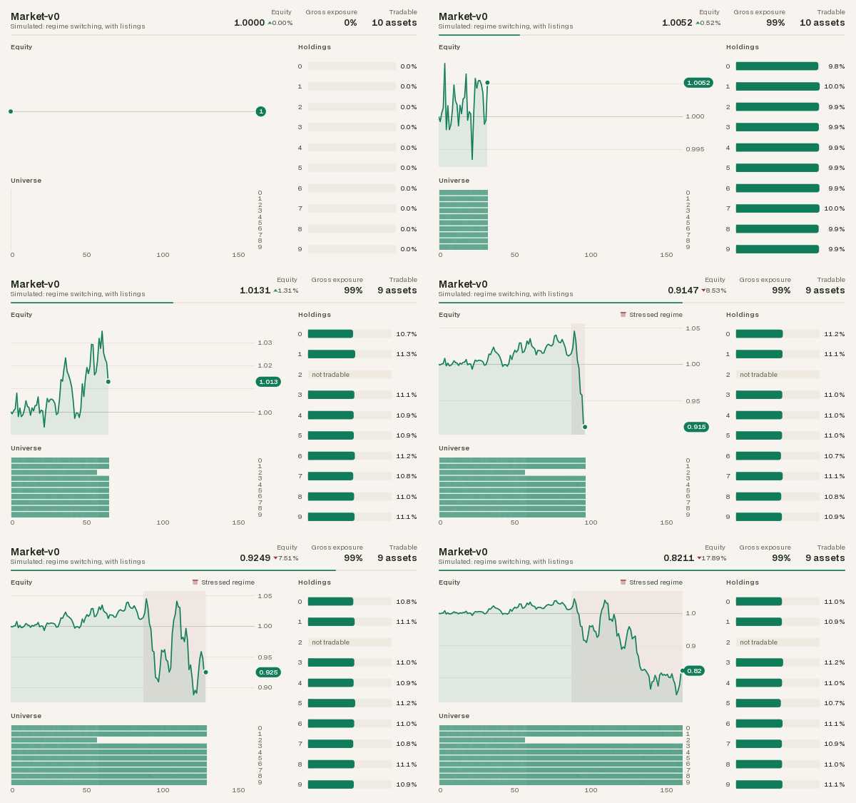
Trade a universe whose members list and delist, with per-asset features, market-wide data,
any cost model, shorting, leverage and financing: the general-purpose environment,
assembled from the finance toolkit. The class is
sekai.envs.finance.MarketEnv.
Data. Either a historical MarketData (data=; NaN prices mark
unlisted assets, and episodes are windows chosen by sampler or
reset(options={"start": ...})), or a market model (model=)
that simulates a new market every episode. The default, default_market(), is ten assets
in a two-regime market: calm (8% drift, 15% volatility, pairwise correlation 0.2) and
stressed (−20%, 40%, 0.7), switching as a hidden Markov chain that stays calm for about two
years and stressed for about six months at a time. Each asset lists at a rate of once a
year and delists at 0.3 a year, with at least two listed, so the tradable set changes
within an episode.
Dynamics. At each decision the action is projected onto the account's rules (long-only
or long/short, gross exposure at most max_leverage, nothing in untradable assets) to give
target weights \(w_t\). Rebalancing from the drifted weights \(\tilde w_t\) costs
\(c_t = C(w_t - \tilde w_t)\) for the cost model \(C\), then the portfolio is held over the
period:
where \(f_t\) is the financing (interest on cash at cash_rate, or margin_rate when it is
borrowed, minus borrow_rate on shorts; see
settlement) and \(R\) the reward function, by
default \(\log g_t\). An asset that delists during the period returns delisting_return and
its position becomes cash.
A NaN price means "not listed", so in a history any gap, even a single missing row (a
trading halt, a data error), counts as a delisting: the position goes to cash at
delisting_return and the slot is freed, and the asset may come back later in another
slot. Fill short gaps first (sekai.finance.features.forward_fill(prices, limit=...)) if
halts should not liquidate positions. Financing accrues once per row with
\(\Delta t\) = dt (weekends and holidays are not accrued separately), and short proceeds
earn the full cash_rate.
| Observation | Dict (below) |
| Action (long-only, default) | Box(0, 1, (max_assets + 1,)) of scores, cash last, normalised into weights summing to max_leverage; all zeros means all cash |
Action (allow_short=True) |
Box(-1, 1, (max_assets,)) of target weights (so each is at most ±1 whatever max_leverage), scaled down if gross exposure \(\sum_i \lvert w_i\rvert\) exceeds max_leverage; the rest is cash |
action_mask() |
int8, 1 for slots tradable now (and for cash, long-only); untradable slots are ignored anyway |
| Reward | reward(outcome), by default the log growth of equity net of costs and financing |
| Termination | equity wiped out |
| Truncation | after episode_length decisions; an episode is a window of an ongoing market, so the observation holds no clock (wrap in TimeAwareObservation(env, max_episode_steps=episode_length) to add one) |
info |
equity, turnover, cost, financing, gross_exposure, n_assets (tradable now), weights (per slot), timestamp (the decision's timestamp in the data; the step index in simulation), dt; and state with privileged_state=True |
The observation is a Dict:
| Key | Space | Content |
|---|---|---|
"assets" |
MaskedBox of max_assets slots, each (lookback, F) |
per asset: the log return, an availability flag (1 where the return is defined), then each field named in features; missing values are 0. "mask" is 1 for slots holding an asset that is tradable now |
"portfolio" |
Box (max_assets + 1,) |
current weights per slot, cash last |
"account" |
Box (2,) |
log equity and gross exposure |
"market" |
Box (lookback, E), only with exogenous |
the market-wide series named in exogenous: MarketData exogenous series, or model state such as "regime" |
A MaskedBox is a Dict with "values" and "mask" keys, so every Dict utility,
wrapper and the gymnasium bridge handle it; NormalizeObservation normalises it per
feature over occupied slots only (see the dynamic observations guide).
| Parameter | Default | Meaning |
|---|---|---|
data |
None |
historical MarketData |
model |
default_market() |
market model when there is no data |
max_assets |
every asset | slots in the observation and action |
features |
() |
per-asset data fields to observe (needs data) |
exogenous |
() |
market-wide series to observe: MarketData exogenous names, or model state keys |
lookback |
20 |
rows in each observation window |
episode_length |
252 |
decisions per episode |
sampler |
"random" |
where episodes start in the history |
transaction_cost |
1e-3 |
a rate or a CostModel, priced per asset (per-asset rates follow the data's columns); uses the data's volume (shares) and spread (fraction of the price) fields when present |
reward |
LogReturn() |
a RewardFunction |
allow_short |
False |
long/short action space |
max_leverage |
1.0 |
cap on gross exposure |
cash_rate, margin_rate, borrow_rate |
0.0, cash_rate, 0.0 |
annual rates on cash, borrowed cash and shorts |
capital |
1_000_000 |
account size in currency, for costs that need it |
dt |
from the data | years per step: 1 / data.periods_per_year, the model's dt, or 1/252 |
delisting_return |
0.0 |
return of an asset over the period in which it delists |
privileged_state |
False |
add the simulation's latent state at the decision time to info["state"] |
market = sekai.make("Market-v0")
result = market.reset(seed=0)
print(result.observation["assets"]["values"].shape, result.observation["assets"]["mask"])  # (10, 20, 2) [1 1 0 1 1 1 1 0 1 1]
print(market.action_mask())  # [1 1 0 1 1 1 1 0 1 1 1]
print(market.action_space.sample(mask=market.action_mask())[[2, 7]])  # [0. 0.]
Slots and dynamic universes
With max_assets=None each asset has its own slot. A long history can hold many more
assets than are ever listed at once; a smaller max_assets then maps them to slots with a
SlotMap (sekai.finance.universe): an asset keeps its slot as long as it is tradable,
newcomers take the lowest free slots (incumbents first, then in column order), and while
every slot is taken further newcomers wait. A slot that changes hands starts with weight
zero, so per-slot features, normalisation statistics and recurrent state are never mixed
between two assets without the mask showing it. env.slot_assets names each slot's
asset.
Thirty stocks over 2,520 weekdays, between 10 and 19 listed on any day, in 16 slots, with a momentum feature and a 5 bp half-spread:
from sekai.finance import ListingProcess
from sekai.finance.features import momentum

rng = np.random.default_rng(0)
universe = ListingProcess(GBM(mu=rng.uniform(-0.05, 0.15, 30), sigma=rng.uniform(0.15, 0.45, 30)),
                          initial_listed=0.4, listing_rate=0.3, delisting_rate=0.3, min_listed=4)
sim = universe.simulate(rng, 2519)
stocks = MarketData(sim.prices, timestamps=np.busday_offset("2015-01-01", np.arange(2520), roll="forward"),
                    assets=[f"STK{i:02d}" for i in range(30)])
stocks = stocks.with_fields(momentum=np.tanh(10 * momentum(stocks.prices, 60)))
print(stocks.mask.sum(axis=1).min(), stocks.mask.sum(axis=1).max())  # 10 19

env = sekai.make("Market-v0", data=stocks, max_assets=16, features=["momentum"], lookback=20,
                 transaction_cost=SpreadCost(half_spread=5e-4))
print(env.observation_space["assets"])  # MaskedBox(-inf, inf, (20, 3), max_size=16, float32)
result = env.reset(seed=0)
print(result.info["timestamp"], env.slot_assets[12:])  # 2022-05-30 ('STK18', 'STK19', 'STK22', 'STK23')
for _ in range(100):
    result = env.step(np.append(env.action_mask()[:-1], 0.0).astype(np.float32))
print(result.info["timestamp"], env.slot_assets[12:])  # 2022-10-17 ('STK18', 'STK28', None, 'STK23')
STK19 left and STK28 took its slot; STK22's slot is empty. On its own:
from sekai.finance import SlotMap

slots = SlotMap(3)
print(slots.update(["AAPL", "MSFT"]))  # [0 1]
print(slots.update(["MSFT", "NVDA", "AMZN"]), slots.assets, slots.changed)  # [1 0 2] ('NVDA', 'MSFT', 'AMZN') [ True False  True]
Baselines. Market-v0 builds a padded multi-asset observation every step, so it is
slower than the environments above (about 10,000 steps a second); its baselines use the
first 50 seeds. On the default simulated market, with the regime made observable for the
oracle:
def equal_weight(env, obs):
    return np.append(env.action_mask()[:-1], 0.0).astype(np.float32)  # tradable assets, no cash


def regime_oracle(env, obs):  # sees the hidden regime: cash while stressed
    stressed = obs["market"][-1, 0] == 1.0
    return np.eye(11, dtype=np.float32)[10] if stressed else equal_weight(env, obs)


market = sekai.make("Market-v0", exogenous=["regime"])
market.action_space.seed(0)
for name, policy in {
    "equal weight": equal_weight,
    "regime oracle": regime_oracle,
    "all cash": lambda env, obs: np.eye(11, dtype=np.float32)[10],
    "random": lambda env, obs: env.action_space.sample(mask=env.action_mask()),
}.items():
    print(f"{name:14s} {evaluate(market, policy, episodes=50)}")
equal weight   +0.0129 ± 0.1783
regime oracle  +0.0516 ± 0.0689
all cash       +0.0000 ± 0.0000
random         -0.1313 ± 0.1590
The stressed regime wipes out most of the calm regime's drift for an always-invested portfolio. Knowing the regime is worth about 4% a year and cuts the dispersion by more than half; a learned policy has to infer it from returns and correlations, and is bounded by the oracle. On the thirty-stock history, where drifts differ persistently between stocks:
def momentum_tilt(env, obs):
    values, mask = obs["assets"]["values"], obs["assets"]["mask"]
    score = np.where(mask == 1, np.exp(3 * values[:, -1, 2]), 0.0)  # latest momentum feature
    return np.append(score, 0.0).astype(np.float32)


env.action_space.seed(0)
for name, policy in {
    "equal weight": equal_weight,
    "momentum tilt": momentum_tilt,
    "random": lambda env, obs: env.action_space.sample(mask=env.action_mask()),
}.items():
    print(f"{name:14s} {evaluate(env, policy, episodes=50)}")
MarketMaking-v0
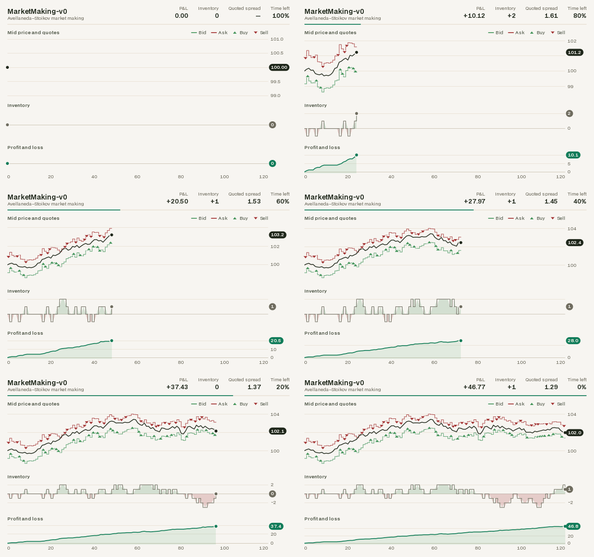
Quote a bid and an ask around a moving mid price, earning the spread while managing inventory risk: the market-making model of Avellaneda & Stoikov (2008), with the parameters of the paper's numerical example.
Dynamics. The session \([0, T]\) is split into \(N\) steps of \(\Delta t = T/N\). The mid price is an arithmetic Brownian motion:
The agent quotes a bid at \(S_t - \delta^b\) and an ask at \(S_t + \delta^a\). Each side is filled within the step, independently, with probability
for order_size units at the quoted price. A side is not quoted while the inventory \(q\) is
at its limit on that side. With cash \(X_t\), the reward is the change in mark-to-market
wealth minus a running inventory penalty:
Closed-form quotes. For this model Avellaneda and Stoikov derive (approximately) optimal quotes, centred on a reservation price \(r = S - q\gamma\sigma^2 (T - t)\) that is skewed against the inventory, with total spread
env.avellaneda_stoikov_action() returns these distances, clipped to [0, max_offset], for
the current state.
| Observation | Box([-1, 0], [1, 1], (2,), float32): inventory / max_inventory and the fraction of the session remaining (the model's Markov state; the price level does not affect optimal quotes) |
| Action | Box(0, max_offset, (2,), float32): bid and ask distances from the mid |
| Reward | change in mark-to-market wealth minus the inventory penalty |
| Termination | at the end of the session (n_steps steps); the clock is observed, so this is a true terminal state |
info |
mid_price, inventory, cash, wealth, bid, ask, bid_filled, ask_filled (bid/ask are NaN after reset()), timestamp (session time), dt (\(\Delta t\)) |
| Parameter | Default | Symbol |
|---|---|---|
s0 |
100.0 |
\(S_0\) |
sigma |
2.0 |
\(\sigma\) |
total_time |
1.0 |
\(T\) |
n_steps |
200 |
\(N\) (\(\Delta t = 0.005\)) |
fill_intensity |
140.0 |
\(A\) |
fill_decay |
1.5 |
\(k\) |
risk_aversion |
0.1 |
\(\gamma\) |
max_inventory |
50 |
inventory limit, either side |
order_size |
1 |
units per fill |
max_offset |
5.0 |
largest quote distance |
The env also exposes wealth, time_remaining and fill_probability(offset):
mm = sekai.make("MarketMaking-v0")
mm.reset(seed=0)
print(mm.avellaneda_stoikov_action())  # [0.8453852 0.8453852]
print(round(mm.fill_probability(0.0), 3), round(mm.fill_probability(1.0), 3))  # 0.503 0.145
Baselines (episode return = risk-adjusted P&L):
for name, policy in {
    "Avellaneda-Stoikov": lambda env, obs: env.avellaneda_stoikov_action(),
    "fixed 0.5 / 0.5": lambda env, obs: np.full(2, 0.5, np.float32),
    "fixed 1.0 / 1.0": lambda env, obs: np.full(2, 1.0, np.float32),
    "fixed 2.0 / 2.0": lambda env, obs: np.full(2, 2.0, np.float32),
}.items():
    print(f"{name:19s} {evaluate(mm, policy)}")
Avellaneda-Stoikov  +56.7591 ± 6.6943
fixed 0.5 / 0.5     +48.6030 ± 17.5252
fixed 1.0 / 1.0     +51.7827 ± 14.3403
fixed 2.0 / 2.0     +25.7799 ± 8.6182
The inventory-aware quotes earn more, with less than half the dispersion of the best
symmetric quote. make() adds no wrappers to the finance environments, so methods such as
avellaneda_stoikov_action() can be called on the env directly; once you wrap it, call them
on env.unwrapped.
OptimalExecution-v0
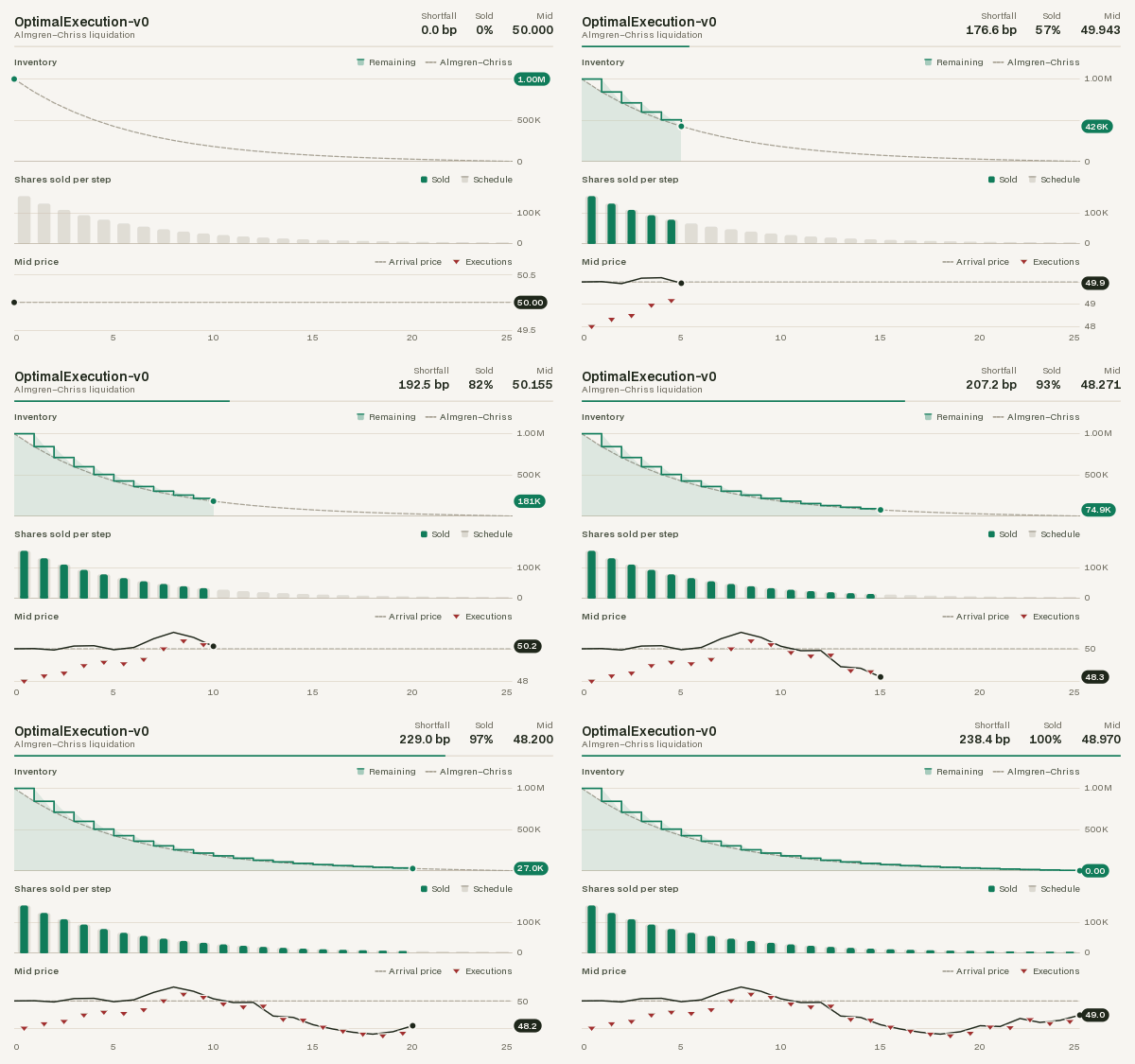
Liquidate a large position over a fixed horizon, trading off market impact (sell fast and you move the price) against risk (sell slowly and the price may move against you): the execution model of Almgren & Chriss (2000), with the defaults of the paper's example, one million shares of a $50 stock over five days.
Dynamics. The horizon \(T\) is split into \(N\) periods of \(\tau = T/N\). Holding \(x_k\) shares, the agent sells \(n_k\) in period \(k\) at the execution price
and the mid then moves by volatility and permanent impact:
The reward, in basis points of the arrival notional \(X S_0\), is
so the episode return is minus the Almgren–Chriss mean-variance objective: the implementation shortfall plus \(\lambda\) times its variance proxy \(\sigma^2\tau\sum_k x_k^2\).
Closed-form schedule. With \(\tilde\eta = \eta - \tfrac12\gamma\tau\) and \(\tilde\kappa^2 = \lambda\sigma^2/\tilde\eta\), the optimal holdings are
which reduces to the straight line of TWAP when \(\lambda = 0\). For any static schedule, the shortfall has mean and variance
| Method | Returns |
|---|---|
almgren_chriss_trajectory() |
optimal holdings \(x_0, \dots, x_N\) (x_0 = X, x_N = 0), evaluated (with the arsinh form of \(\kappa\)) so that it stays finite however large \(\kappa T\) is and tends to TWAP as \(\lambda \to 0\) |
almgren_chriss_actions() |
the same schedule as actions, shape (N, 1) |
expected_shortfall(trades) |
closed-form (mean, variance) of the shortfall of a static schedule |
| Observation | Box(3,): remaining inventory / \(X\), the fraction of the horizon remaining, and the mid's move since arrival in units of \(\sigma\sqrt{T}\) |
| Action | Box(0, 1, (1,), float32): the fraction of the remaining inventory to sell this period; whatever is left is sold in the last period regardless |
| Reward | as above, in bps |
| Termination | inventory fully sold, or the horizon reached |
info |
shares_sold, execution_price, inventory, mid_price, implementation_shortfall (dollars, cumulative), shortfall_bps, timestamp (time since arrival), dt (\(\tau\)) |
| Parameter | Default | Symbol |
|---|---|---|
initial_inventory |
1e6 |
\(X\) (shares) |
s0 |
50.0 |
\(S_0\) |
sigma |
0.95 |
\(\sigma\) ($/share/day\(^{1/2}\)) |
total_time |
5.0 |
\(T\) (days) |
n_steps |
25 |
\(N\) (\(\tau = 0.2\) days) |
permanent_impact |
2.5e-7 |
\(\gamma\) |
temporary_impact |
2.5e-6 |
\(\eta\) (must exceed \(\gamma\tau/2\)) |
fixed_cost |
0.0625 |
\(\epsilon\) (half the bid-ask spread) |
risk_aversion |
1e-6 |
\(\lambda\) |
Baselines. Every finance env exposes the step index as env.elapsed_steps, which
schedule-based policies need:
env = sekai.make("OptimalExecution-v0")
n = env.n_steps
schedule = env.almgren_chriss_actions()

for name, policy in {
    "Almgren-Chriss": lambda env, obs: schedule[env.elapsed_steps],
    "TWAP": lambda env, obs: np.array([1.0 / (n - env.elapsed_steps)], np.float32),
    "sell at once": lambda env, obs: np.ones(1, np.float32),
}.items():
    print(f"{name:15s} {evaluate(env, policy)}")
TWAP has the lowest expected impact cost but carries the most risk; the Almgren–Chriss schedule front-loads selling and wins on the mean-variance objective the reward measures. The simulator agrees with the closed form:
holdings = env.almgren_chriss_trajectory()
mean, var = env.expected_shortfall(holdings[:-1] - holdings[1:])
print(f"closed form: E[IS] = ${mean:,.0f}, sd = ${np.sqrt(var):,.0f}")  # closed form: E[IS] = $958,704, sd = $801,877

shortfalls = []
for seed in range(2000):
    result = env.reset(seed=seed)
    while not result.done:
        result = env.step(schedule[env.elapsed_steps])
    shortfalls.append(result.info["implementation_shortfall"])
print(f"simulated:   E[IS] = ${np.mean(shortfalls):,.0f}, sd = ${np.std(shortfalls):,.0f}")  # simulated:   E[IS] = $951,425, sd = $780,690
LimitOrderBook-v0
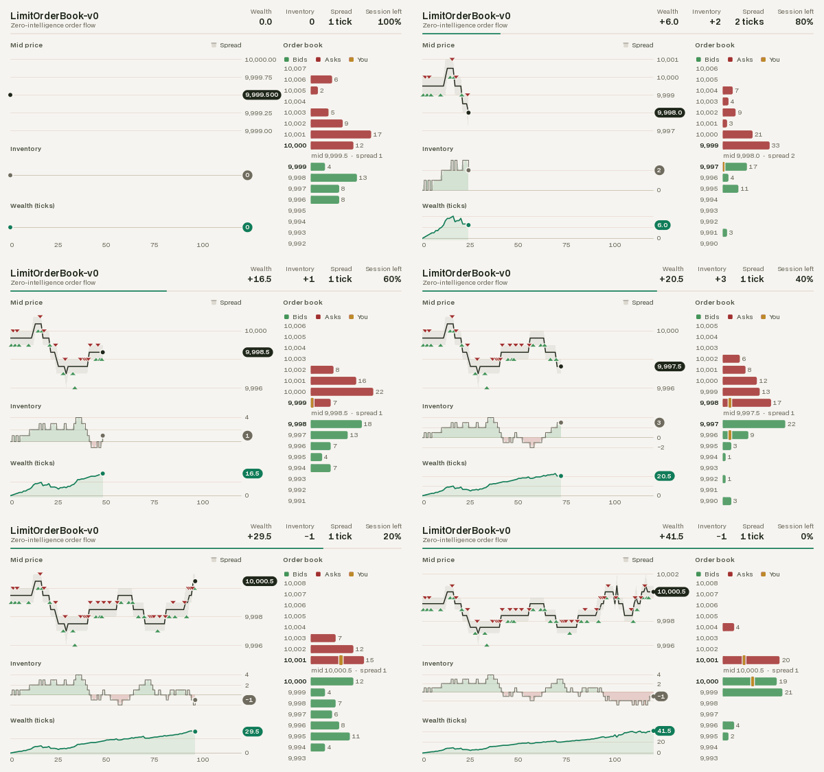
Make markets, or trade, in a simulated limit order book: the microstructure counterpart of
MarketMaking-v0. Where that environment draws fills from a formula, here the agent's
quotes rest in a real price-time priority order book against
background traders, so queue position, the spread and the depth all emerge from the order
flow. The class is sekai.envs.finance.LimitOrderBookEnv.
Dynamics. Each episode seeds a book around mid_price and lets the background flow (a
ZeroIntelligenceFlow: Poisson
limit orders, market orders and cancellations) run for warmup time units. Then, every
\(\Delta\) = decision_interval units of time until session_length, the agent
- optionally sends a market order of
order_sizelots, after cancelling its own resting quote on the opposite side: a market buy first cancels the agent's ask, a market sell its bid. This is self-trade prevention, as in the cancel-resting mode of most exchanges: the agent never trades with itself; - places, keeps, moves or cancels one bid and one ask (a quote left at the same price keeps its place in the queue; moving it sends it to the back; repeating an action keeps a quote that is still at that level, including a level-1 quote alone at the best price; a quote cancelled in step 1 is placed again, at the back of its queue, unless its level is 0),
and the book evolves through however many background events occur before the next decision, which may fill the agent's resting quotes. With cash \(X_t\) and inventory \(q_t\) in lots, marked at the mid \(m_t\) (all prices in ticks), the reward is
the change in mark-to-market wealth minus a running inventory penalty at rate
\(\phi\) = inventory_penalty per squared lot per unit of time.
| Observation | Dict (below) |
| Action | MultiDiscrete([K + 1, K + 1, 3]), \(K\) = max_quote_offset: the bid level (0 = no bid, 1 = join the best bid of the other traders, \(k\) = \(k - 1\) ticks behind it), the ask level (likewise), and a market order (0 sell, 1 none, 2 buy), which first cancels the agent's own quote on the opposite side (self-trade prevention). A resting quote already at the requested level stays where it is with its queue position, and a level-1 quote stays put while it is itself the best price, even alone there, so an unchanged action only moves a quote to follow the other traders' best price |
action_mask() |
a tuple of per-dimension int8 masks: at the long inventory limit no bid and no market buy, at the short limit no ask and no market sell |
| Reward | change in mark-to-market wealth (ticks) minus the inventory penalty |
| Termination | at the end of the session (n_steps = session_length / decision_interval decisions); the clock is observed |
info |
timestamp (session time), dt (the time the step covered: decision_interval, or less on a final, shorter step), mid_price, spread, inventory, cash, wealth, fills (the agent's fills this step) |
| Key | Space | Content |
|---|---|---|
"book" |
Box (levels, 4) |
for the best levels price levels: bid price minus the mid (ticks), bid size, ask price minus the mid, ask size; zeros for missing levels |
"trades" |
MaskedBox of max_trades slots, each (3,) |
the most recent trades, oldest first: price minus the current mid, size, aggressor side (+1 buy, -1 sell); a variable-size set |
"agent" |
Box (6,) |
inventory / max_inventory, fraction of the session remaining, whether a bid and an ask are resting, and the volume queued ahead of each |
| Parameter | Default | Meaning |
|---|---|---|
flow |
ZeroIntelligenceFlow() |
background order flow |
mid_price |
10_000 |
initial mid price in ticks |
session_length |
300.0 |
session length, in the flow's time units |
decision_interval |
1.0 |
time between decisions (\(\Delta\)) |
levels |
5 |
book levels observed |
max_quote_offset |
5 |
farthest quote level \(K\) |
order_size |
1 |
lots per quote or market order |
max_inventory |
20 |
inventory limit, either side |
inventory_penalty |
0.01 |
\(\phi\), per squared lot per unit of time |
max_trades |
16 |
recent trades in the observation |
warmup |
20.0 |
time the book evolves before the session starts |
lob = sekai.make("LimitOrderBook-v0")
result = lob.reset(seed=0)
print(result.observation["book"][0])  # [-0.5  9.   0.5  8. ]
print(result.info["mid_price"], result.info["spread"], lob.n_steps)  # 10000.5 1 300
env.book is the live OrderBook, for analysis (do not modify it).
Baselines. The order book simulates every background event in Python, about 6,000 decisions a second, so these use the first 50 seeds:
JOIN, BEHIND, NO_QUOTE, NO_MARKET_ORDER = 1, 3, 0, 1


def inventory_skew(env, obs):
    """Join the best quote on the side that reduces inventory, stay two ticks behind on the other."""
    q = obs["agent"][0]
    return np.array([JOIN if q <= 0 else BEHIND, JOIN if q >= 0 else BEHIND, NO_MARKET_ORDER])


lob.action_space.seed(0)
for name, policy in {
    "inventory skew": inventory_skew,
    "join both quotes": lambda env, obs: np.array([JOIN, JOIN, NO_MARKET_ORDER]),
    "no quotes": lambda env, obs: np.array([NO_QUOTE, NO_QUOTE, NO_MARKET_ORDER]),
    "random": lambda env, obs: env.action_space.sample(mask=env.action_mask()),
}.items():
    print(f"{name:17s} {evaluate(lob, policy, episodes=50)}")
inventory skew    +86.2148 ± 7.0613
join both quotes  -1.7224 ± 131.6676
no quotes         +0.0000 ± 0.0000
random            -393.1354 ± 235.4022
Quoting both sides at the touch earns the spread but lets inventory random-walk with the order flow, so its P&L is dominated by the price moves it is exposed to. Leaning the quotes against inventory, a crude form of the Avellaneda–Stoikov skew, keeps inventory near zero and turns the spread into a steady profit. A learned policy can also use the queue positions and recent trades it observes.
LimitOrderBookMarket
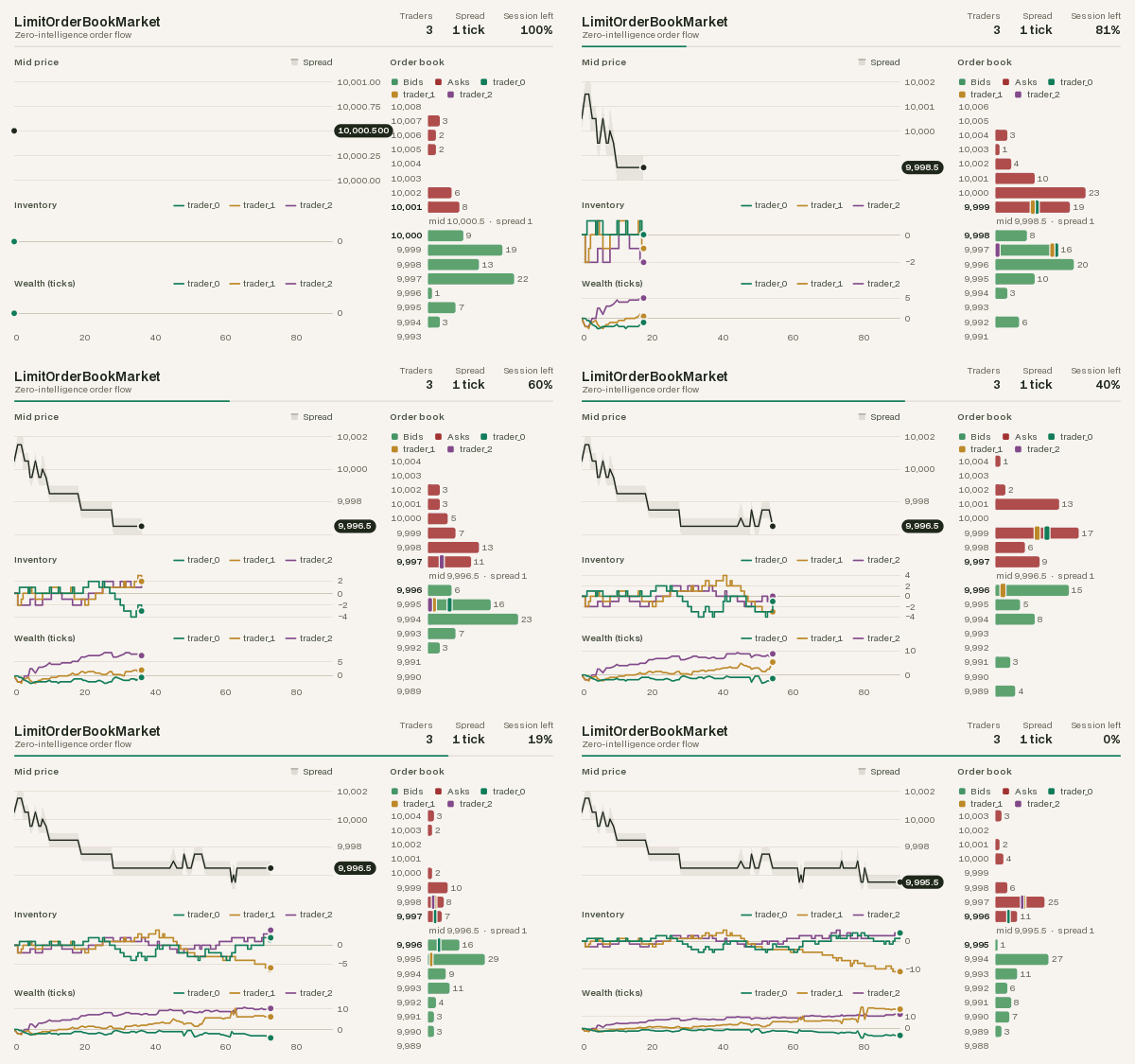
Several RL traders in one order book, each deciding on its own clock: an
event-driven multi-agent environment
(sekai.envs.finance.LimitOrderBookMarket, a sekai.MultiAgentEnv; construct it
directly). One trader's market order can fill another's resting quote (never its own:
self-trade prevention applies to every trader), so the traders compete for the spread and
for queue priority as well as against the background flow.
LimitOrderBookMarket(n_agents=2, *, decision_intervals=1.0, jitter=0.0, **market) names
its traders "trader_0", "trader_1", ...; trader \(i\) decides every
decision_intervals[i] units of time (one value for all, or one per trader), each wait
multiplied by a random factor in \([1 - \text{jitter}, 1 + \text{jitter}]\). The other
arguments (flow, mid_price, session_length, levels, max_quote_offset,
order_size, max_inventory, inventory_penalty, max_trades, warmup) are as for
LimitOrderBook-v0, and so are each trader's observation, action, action_mask(agent) and
reward.
Each step(actions) takes actions from exactly the traders whose turn it is, checks them all
(an invalid one raises InvalidAction before any is carried out, so the failed step changes
nothing), carries them out in name order, then advances the book to the next decision time
of any trader, and returns:
observationsonly for the traders that act next: the keys say who moves;rewards,terminated,truncatedandinfofor every trader, so rewards earned between a trader's decisions are not lost: sum them until its next observation. The inventory penalty is charged for the time each step covers, whichinfo[agent]["dt"]reports;info[agent]["acting"]says whether that trader acts next.
When several traders' decision times coincide they act in name order, so trader_0's
quotes reach the book (and the queue) first. At the end of the session every trader is
terminated and observed; agents is then empty, and step() raises ResetRequired until
the next reset().
from sekai.envs.finance import LimitOrderBookMarket

lobm = LimitOrderBookMarket(n_agents=3, decision_intervals=[1.0, 2.0, 5.0], jitter=0.1)
result = lobm.reset(seed=0)
print(sorted(result.observations))  # ['trader_0', 'trader_1', 'trader_2']
returns = dict.fromkeys(lobm.possible_agents, 0.0)
decisions = dict.fromkeys(lobm.possible_agents, 0)
while lobm.agents:
    actions = {agent: inventory_skew(lobm, obs) for agent, obs in result.observations.items()}
    for agent in actions:
        decisions[agent] += 1
    result = lobm.step(actions)
    for agent, reward in result.rewards.items():
        returns[agent] += reward
print(decisions)
print({agent: round(total, 1) for agent, total in returns.items()})
{'trader_0': 302, 'trader_1': 150, 'trader_2': 60}
{'trader_0': 89.8, 'trader_1': 73.8, 'trader_2': 43.6}
sekai.compat.to_pettingzoo converts it to a PettingZoo
parallel environment, in which only the acting traders appear in each observation dict.
Native vector environments
Trading-v0, Portfolio-v0, MarketMaking-v0 and OptimalExecution-v0 have natively
vectorised versions in sekai.envs.finance. Each simulates num_envs copies with array
operations, so one step() advances every sub-env at once, and sekai.make_vec uses them
by default (sekai list marks these environments [native vec]):
| ID | Class | Batched helpers |
|---|---|---|
Trading-v0 |
TradingVecEnv |
|
Portfolio-v0 |
PortfolioVecEnv |
action_to_weights(actions): (num_envs, n_assets + 1) targets |
MarketMaking-v0 |
MarketMakingVecEnv |
avellaneda_stoikov_action(): (num_envs, 2) quotes; wealth |
OptimalExecution-v0 |
OptimalExecutionVecEnv |
almgren_chriss_actions(): the (n_steps, 1) schedule, the same for every sub-env |
They take the single environment's keyword arguments and have the same spaces, dynamics,
rewards and info keys, with the vector-env contract of every sekai
VecEnv: batched observations and rewards, same-step autoreset with final_observation,
final_info and reset_info in the infos, an int seed or one per sub-env, and per-env
options. All sub-envs draw from one shared generator, so simulated paths differ draw-for-draw from
the single environments' while being identical in distribution. Each sub-env has its own
copy of the episode sampler, as with every make_vec backend, so a sequential sampler
replays the same windows in every sub-env (to split a history across them, see
Episode samplers); on a history with fixed starts
they reproduce the single environments exactly. Market-v0 and
LimitOrderBook-v0 have no native version; make_vec steps them in a SyncVecEnv (or
pass vectorization_mode="proc" for worker processes). To write a native vector env of
your own, see the vector environments guide.
vec = sekai.make_vec("MarketMaking-v0", 1000)
print(type(vec).__name__)  # MarketMakingVecEnv
result = vec.reset(seed=0)
totals = np.zeros(vec.num_envs)
for _ in range(200):  # every sub-env's session has 200 steps
    result = vec.step(vec.avellaneda_stoikov_action())
    totals += result.rewards
print(f"{totals.mean():+.4f} ± {totals.std():.4f}")  # +56.8336 ± 6.5051

print(type(sekai.make_vec("Portfolio-v0", 4, vectorization_mode="sync")).__name__)  # SyncVecEnv
The same Avellaneda–Stoikov baseline as above, over 1,000 sessions in
one batched run. Passing wrappers= to make_vec selects SyncVecEnv, since a native
env has no per-env objects to wrap; wrap the vector env with Vec* wrappers instead.
Throughput of random actions, measured with sekai bench <id> --num-envs 1024 (native)
and sekai bench <id> --mode sync --num-envs 16 on an 8-core machine (approximate; the
ratio matters more than the absolute numbers):
| ID | Native, 1,024 envs | SyncVecEnv, 16 envs |
Speed-up |
|---|---|---|---|
Trading-v0 |
2,080,000 steps/s | 105,000 steps/s | 20× |
Portfolio-v0 |
910,000 steps/s | 46,000 steps/s | 20× |
MarketMaking-v0 |
2,710,000 steps/s | 105,000 steps/s | 26× |
OptimalExecution-v0 |
2,710,000 steps/s | 139,000 steps/s | 19× |
For comparison, single-environment throughput (sekai bench <id>) is about 9,800 steps/s
for Market-v0 and 6,200 for LimitOrderBook-v0.
Price simulation helpers
sekai.envs.finance exports the simulators the environments use:
| Function | Returns |
|---|---|
simulate_gbm(rng, n_steps, *, s0=100.0, mu=0.0, sigma=0.2, dt=1/252, corr=None) |
GBM paths: shape (n_steps + 1,) for scalar parameters, (n_steps + 1, n) for length-n arrays; row 0 is s0; corr correlates the shocks |
random_correlation(rng, n, strength=0.5) |
a random valid (n, n) correlation matrix |
sample_window(rng, prices, length) |
a random contiguous window of length rows |
from sekai.envs.finance import random_correlation

rng = np.random.default_rng(0)
paths = simulate_gbm(rng, 252, s0=[100, 50], mu=[0.05, 0.1], sigma=[0.2, 0.3],
                     corr=random_correlation(rng, 2))
print(paths.shape, paths[0])  # (253, 2) [100.  50.]
For richer dynamics (stochastic volatility, jumps, regimes, mean reversion, dynamic
universes) see the market simulators; every environment that
takes model= accepts them.